Building Intuition for RL Systems

Understanding the RL System as a Whole

I used to work mostly on large-model pretraining infrastructure. When learning LLM Reinforcement Learning, I spent a huge amount of time on the loss formulas of PPO and GRPO: Why normalize the advantage? What are the numerator and denominator of the importance ratio? Why do we need min and clip? I could explain each of these symbols one by one, but I never really built a complete picture of the RL training process.

It turns out the more effective approach is exactly the opposite: first understand what data the model actually generates, who computes the probabilities, when the weights get updated, and how the updated model changes the next round of data — then derive the loss from these concrete questions. Following this path, I found I could understand RL in the most intuitive way:

1. What’s the difference between the pretraining cross-entropy objective and the RL objective?
2. REINFORCE, baselines, and advantage.
3. Importance sampling and PPO clipping (what exactly is being clipped?), plus GRPO.
4. Understanding what DAPO, Dr.GRPO, and GSPO modify.
5. What causes train–inference inconsistency? Telling policy staleness apart from numerical mismatch.
6. Learning what real RL metrics look like from two Slime runs of Qwen3.5-0.8B on GSM8K.

The key idea running through this whole post is: RL turns the model itself into the generator of its own training data.

The Pretraining Objective vs. the RL Objective

Pretraining: The Samples Are Given

The pretraining objective is usually written as:

$$\mathcal L_{\mathrm{PT}}(\theta)=-\mathbb E_{(x,y)\sim D}\left[\sum_{t=1}^{T}\log\pi_\theta(y_t\mid x,y_{<t})\right].$$

When reading this formula, it helps to start from the innermost part and work outward: $\theta$ denotes all the learnable parameters in the model, $y_t$ is the $t$-th target token, and $y_{<t}$ is the target tokens before it — the prefix the model already knows when predicting the current position. The most important term is $\pi_\theta(y_t\mid x,y_{<t})$: the probability that the model with parameters $\theta$ assigns to the correct next token $y_t$, given context $x$ and prefix $y_{<t}$. The sum $\sum_{t=1}^{T}$ adds up the logprobs at every position in the sequence, and $\mathbb E_{(x,y)\sim D}$ takes the expectation over training samples (approximated by a batch average in practice). Since a higher probability means a higher logprob, the leading minus sign makes “raising the probability of the target token” equivalent to “lowering the loss”.

$\mathcal L_{\mathrm{PT}}(\theta)$ is the pretraining loss to be minimized. $D$ is the distribution of training data; $(x,y)\sim D$ means drawing one sample from it, where $x$ is the given context and $y=(y_1,\ldots,y_T)$ is the target token sequence to predict, with $T$ the target sequence length.

You might wonder: the pretraining objective is usually called cross-entropy. But cross-entropy measures the distance between two distributions — why does this formula appear to contain only a single conditional probability? In fact, two distributions are still present: the model’s predicted distribution, and the one-hot distribution of the ground-truth label (probability $1$ for $y_t$ and $0$ everywhere else). Since all the zero-probability terms vanish from the sum, the formula collapses to a form containing only the conditional probability of $y_t$. This is also documented in 3Blue1Brown’s video on cross-entropy.

The target tokens come from a relatively fixed dataset $D$. Model updates change the probabilities the model assigns to those tokens, but they don’t immediately change which tokens appear in the next batch. In short, the pretraining objective has us fit the model to the distribution of existing data.

RL: The Model Generates Its Own Training Samples

For math RLVR (Reinforcement Learning with Verifiable Rewards), we give the model a problem $x$, let it generate its own answer $y$, and assign a reward $R(x,y)$ via answer checkers, unit tests, and so on:

$$J(\theta)=\mathbb E_{x\sim D_x,\ y\sim\pi_\theta(\cdot\mid x)}[R(x,y)].$$

Here $J(\theta)$ is not a loss to minimize but the RL objective to maximize. $D_x$ is the sampling distribution of problems (prompts); $x\sim D_x$ means first drawing a problem; $\pi_\theta(\cdot\mid x)$ is the probability distribution over all possible answers the model could give for problem $x$, where the "$\cdot$" can be read as a wildcard; $y\sim\pi_\theta(\cdot\mid x)$ means actually sampling one answer from that distribution. $R(x,y)$ is the reward the verifier assigns to “problem $x$ + answer $y$”, and $\mathbb E$ is the expectation over both the drawn problems and the sampled answers. Put differently: we want the answers the model samples by itself to earn a higher reward on average.

This objective maximizes expected reward. The key change is that $y$ no longer comes from static data — it comes from the current policy $\pi_\theta$. So after every update, the distribution of the next round of rollouts shifts too:

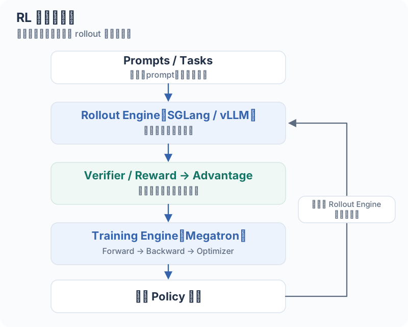
Note that, as you can see in the diagram, the rollout engine here is vLLM / SGLang, because we need to sample $y\sim\pi_\theta(\cdot\mid x)$ — that is, call an inference engine and let the model actually solve the problem. Also notice that this is a feedback loop. Any systematic error tendency, overly long reasoning pattern, sampling bias, or train–inference numerical discrepancy — or in other words, any difference between the distribution of the model used for rollout and the one being trained — can affect the next round of data and then be amplified. This is one of the reasons RL training collapses so easily. It’s also why you hear people discussing the stability of off-policy, async RL and related terms. That’s what the rest of this post covers.

Rollout Is Not Training Forward

In large-model RL, Rollout (inference sampling), Training Forward, and Training Backward actually run on three different sets of kernels:

• RL rollout calls inference engines like SGLang / vLLM: it follows the Prefill + Autoregressive Decode path, relying on operators specifically optimized for low-latency or high-throughput inference, such as Paged KV Cache and Continuous Batching;
• Training Forward calls training engines like Megatron / FSDP: after receiving the complete generated token sequence, it does a whole-sequence forward pass with sequence parallelism, just like pretraining, to recompute logprobs and build the loss;
• Training Backward is a third set of backpropagation operators dedicated to computing derivatives, activation recomputation, and gradient reduction. (Of course, life is much easier when both forward and backward are left to torch.)

Because the underlying operators, tiling strategies, and reduction orders are completely different, nondeterminism or numerical deviation in any of these three kernel sets will cause the computed probabilities or gradients to drift in precision. This means: even in fully synchronous RL — where inference and training use exactly the same model weights $\theta$ — the token probabilities computed by the training forward pass often do not equal the true probabilities the inference engine sampled with at the time. This inherent train–inference mismatch is the main thread we’ll dig into in the second half of this post.

From REINFORCE to Advantage

The Simplest Derivation of the Policy Gradient

To maximize the expected reward $J(\theta)$, we need the gradient $\nabla_\theta J(\theta)$ with respect to the parameters $\theta$. Let’s fix a single problem $x$ and expand the expectation, by definition, into a sum over all possible complete answers $y$:

$$J(\theta)=\mathbb E_{y\sim\pi_\theta(\cdot\mid x)}[R(x,y)] = \sum_y\pi_\theta(y\mid x)R(x,y).$$

But directly differentiating this expression runs into two problems:

1. The reward function $R(x,y)$ is not differentiable: the judge (regexes, unit tests, etc.) is a black box that only scores discrete text; you can’t backpropagate through $R$;
2. The sum $\sum_y$ is intractable: a several-hundred-token answer has an astronomically large space of combinations; enumerating all $y$ is engineering-impossible, so we can only estimate the gradient by sampling a few answers.

To rewrite the gradient back into “an expectation estimable by sampling $y\sim\pi_\theta$”, REINFORCE uses the log-derivative identity $\nabla_\theta \log \pi_\theta = \frac{\nabla_\theta \pi_\theta}{\pi_\theta}$ (i.e., $\nabla_\theta\pi_\theta=\pi_\theta\nabla_\theta\log\pi_\theta$):

$$\begin{aligned} \nabla_\theta J(\theta) &=\sum_y\nabla_\theta\pi_\theta(y\mid x)\,R(x,y)\\ &=\sum_y\pi_\theta(y\mid x)\,\nabla_\theta\log\pi_\theta(y\mid x)\,R(x,y)\\ &=\mathbb E_{y\sim\pi_\theta}\left[R(x,y)\nabla_\theta\log\pi_\theta(y\mid x)\right]. \end{aligned}$$

Look at the middle line: by factoring $\nabla_\theta\pi_\theta$ into $\pi_\theta \cdot \nabla_\theta\log\pi_\theta$, we’ve reconstructed the probability distribution $\pi_\theta(y\mid x)$, so the weighted sum over all $y$, $\sum_y \pi_\theta(y\mid x)[\dots]$, naturally turns back into the expectation $\mathbb E_{y\sim\pi_\theta}[\dots]$.

This transformation solves both problems at once:

• No need to differentiate $R(x,y)$: the gradient operator $\nabla_\theta$ acts only on the model’s own generation probability $\log\pi_\theta(y\mid x)$ (called the score function); $R(x,y)$ is just a scalar weight;
• Sampling replaces enumeration: since it’s an expectation $\mathbb E_{y\sim\pi_\theta}$, we just let the model roll out and sample a few answers $y$, compute their $\nabla_\theta\log\pi_\theta(y\mid x)$, multiply by the corresponding rewards $R(x,y)$, and we obtain an unbiased estimate of the gradient direction.

The logprob of a complete answer decomposes as:

$$\log\pi_\theta(y\mid x)=\sum_{t=1}^T\log\pi_\theta(y_t\mid x,y_{<t}).$$

Here the $\pi_\theta(y\mid x)$ on the left is the joint probability of the entire answer; the right-hand side expands it into the conditional probabilities of generating each next token — the chain rule of probability. For brevity later, we’ll refer to “prompt $x$ plus the first $t-1$ generated tokens” collectively as $h_t=(x,y_{<t})$, so $\pi_\theta(y_t\mid h_t)$ denotes the same conditional probability. Compare with the pretraining objective

$$\mathcal L_{\mathrm{PT}}(\theta)=-\mathbb E_{(x,y)\sim D}\left[\sum_{t=1}^{T}\log\pi_\theta(y_t\mid x,y_{<t})\right].$$

The two look strikingly similar. The differences come down to two points: (1) REINFORCE looks just like reward-weighted cross-entropy on the tokens the model itself generated; (2) here we estimate the policy gradient by sampling, not by backpropagating directly through the non-differentiable sampling operation.

Are Wrong Answers Punished?

If the correctness reward is $R\in\{0,1\}$ and we directly use the single-sample objective $-R\log\pi_\theta(y\mid x)$, then when the answer is wrong and $R=0$:

$$\nabla_\theta\mathcal L=-R\nabla_\theta\log\pi_\theta(y\mid x)=0.$$

A wrong answer has no direct gradient. It is not the case that “the reward is zero, so the model will still push down the probability of wrong answers”. The signal we actually want is: answers better than expected should be encouraged, and answers worse than expected should be suppressed. This naturally leads to the notion of advantage we’ll introduce next.

Where Advantage Comes From

Define $A(x,y)=R(x,y)-b(x)$, where $b(x)$ depends only on the prompt, not on the sampled answer itself. Then: $A$ is the advantage, measuring whether the answer’s reward is above or below a reference level; $b(x)$ is that reference level — the baseline. It doesn’t have to be $0$, and it doesn’t have to come from another model; for example, it can be the expected reward on this problem. We write $b(x)$ rather than $b(x,y)$ to emphasize: once the problem is fixed, it must not vary with the current sampled response — otherwise the derivation below, “subtracting it doesn’t change the expected gradient”, breaks down (as you’ll see, if $b$ depends on the distribution, we can’t factor it out):

$$\begin{aligned} \mathbb E_{y\sim\pi_\theta}[b(x)\nabla\log\pi_\theta(y\mid x)] &=b(x)\sum_y\nabla\pi_\theta(y\mid x)\\ &=b(x)\nabla 1=0. \end{aligned}$$

So $\mathbb E[R\nabla\log\pi]=\mathbb E[(R-b)\nabla\log\pi]$. A well-chosen baseline leaves the expected policy gradient unchanged while reducing estimation variance.

• $A>0$: increase the logprob of this sampled answer.
• $A<0$: decrease the logprob of this answer.
• $A=0$: this sample carries no policy-gradient signal.

How GRPO Estimates Advantage

Actor–Critic methods can train $V^\pi(x)$ to serve as the baseline (this is what PPO does), but GRPO needs no extra critic. For each prompt it samples $G$ answers and uses the mean and standard deviation of the group’s rewards:

$$A_i=\frac{R_i-\bar R}{\sigma_R+\epsilon}.$$

Here $G$ is the number of answers sampled per prompt, $i\in\{1,\ldots,G\}$ is the answer index, and $R_i=R(x,y_i)$ is the reward of the $i$-th answer. $\bar R=(1/G)\sum_{i=1}^{G}R_i$ is the group’s mean reward and $\sigma_R$ is the standard deviation of those $G$ rewards; the numerator $R_i-\bar R$ measures how much better than the group average this answer is. $\epsilon$ is a tiny constant that prevents division by zero when $\sigma_R=0$ (note: it shares its name with the $\epsilon$ in PPO clipping later, but its purpose is completely different). So this formula does two things: first compute relative performance, then rescale by within-group variability.

For example, with 8 answers of which 2 are correct and 6 wrong:

$$\bar R=0.25,\qquad\sigma_R=\sqrt{0.25\times0.75}\approx0.433.$$

Answer	Mean-only $R-\bar R$	GRPO advantage after dividing by std
Correct	$+0.75$	$+1.732$
Wrong	$-0.25$	$-0.577$

So we can both encourage correct answers and directly suppress wrong ones.

Notably, for binary rewards, an all-correct or all-wrong group has $\sigma_R=0$ and all centered advantages are zero; implementations must handle the $\epsilon$ in the denominator carefully, but it cannot manufacture a learning signal — as you’ll see later, this is exactly what DAPO addresses.

Importance Ratios and PPO Clipping

Why “Sample from the Old Policy, Train the New” Needs Correction

The objective is an expectation under the current policy, but a batch of samples usually comes from the old policy $\pi_{\mathrm{old}}$ that was live at sampling time. For a fixed prefix $h$ and token $a$:

$$\begin{aligned} \mathbb E_{a\sim\pi_\theta}[f(a)] &=\sum_a\pi_{\mathrm{old}}(a\mid h)\frac{\pi_\theta(a\mid h)}{\pi_{\mathrm{old}}(a\mid h)}f(a)\\ &=\mathbb E_{a\sim\pi_{\mathrm{old}}}[r(a\mid h)f(a)],\\ \text{where }r(a\mid h)&=\frac{\pi_\theta(a\mid h)}{\pi_{\mathrm{old}}(a\mid h)}. \end{aligned}$$

This time we focus on one fixed generation prefix $h$: $a$ is a possible next token (or action), $\pi_{\mathrm{old}}(a\mid h)$ is the probability the old policy at sampling time assigned to it, and $\pi_\theta(a\mid h)$ is the probability under the current policy. $f(a)$ is any quantity we want to take the expectation of; $\sum_a$ adds up the contributions of all possible tokens in the vocabulary. $r(a\mid h)$ is the importance ratio: how much more likely the new policy considers this token, relative to the old one. The key to the identity is “multiply by the old probability, then divide by the old probability”, which lets us estimate an expectation under the new policy from old-policy samples; it requires the denominator to be nonzero wherever it matters.

For example: if the old policy gives a token probability $0.1$ and the current policy gives $0.2$, then $r=2$ — that sample from the old distribution needs to be scaled up 2× when estimating the expectation under the new distribution. This presupposes that the old distribution covers the support of the new one.

But note: the strict importance ratio of an entire autoregressive trajectory is the product of all per-token ratios:

$$\frac{\pi_\theta(y\mid x)}{\pi_{\mathrm{old}}(y\mid x)} =\prod_{t=1}^{T}\frac{\pi_\theta(y_t\mid h_t)}{\pi_{\mathrm{old}}(y_t\mid h_t)}.$$

$\prod_{t=1}^{T}$ is a product (the multiplicative counterpart of the earlier $\sum$); each $h_t$ is the actual prefix before that token. Since the probability of a whole answer equals the product of per-token conditional probabilities, the importance ratio of a whole trajectory also multiplies the per-token ratios.

Why doesn’t actual training use this product ratio directly? Imagine a reasoning answer of length $T=1000$ tokens: even if each token’s new/old probability ratio fluctuates by only $1\%$, the product becomes $1.01^{1000}\approx 20959$ or $0.99^{1000}\approx 0.00004$, making the gradient variance explode or vanish outright. So PPO/GRPO abandon the strict whole-trajectory product and settle for approximating importance sampling at the individual token level — each position only looks at its own single-step ratio $r_t=\pi_\theta(y_t\mid h_t)/\pi_{\mathrm{old}}(y_t\mid h_t)$.

What Does PPO’s Clipping Actually Clip?

Even after switching to the per-token ratio $r_t$, directly maximizing the unclipped objective $r_t A_t$ still causes trouble: whenever a token’s advantage $A_t>0$, the model will push $r_t$ toward infinity to score high — in other words, it has an incentive to drift as far from the original distribution as possible. But once $\pi_\theta$ strays too far from $\pi_{\mathrm{old}}$, gradients estimated from old samples are no longer trustworthy.

So we need a brake that knows when to stop: once $r_t$ deviates from $1$ by more than a tolerance $\epsilon$ (e.g., $\epsilon=0.2$, i.e., the legal range is $[0.8, 1.2]$), we stop providing gradient for it. This is the clipped surrogate objective that PPO maximizes:

$$\boxed{L^{\mathrm{CLIP}}_t(\theta)=\min\big(r_tA_t,\ \operatorname{clip}(r_t,1-\epsilon,1+\epsilon)A_t\big).}$$

First, the symbols:

• $r_t=\pi_\theta(y_t\mid h_t)/\pi_{\mathrm{old}}(y_t\mid h_t)$ is the new/old policy probability ratio for the $t$-th token;
• $A_t$ is the advantage assigned to that token (in outcome-level GRPO, all tokens in the same answer usually share the same $A_i$);
• $\operatorname{clip}(r_t, 1-\epsilon, 1+\epsilon)$ forcibly flattens any $r_t$ outside $[1-\epsilon, 1+\epsilon]$ to the boundary constant. Note that once the function is flattened to a constant, its gradient with respect to $\theta$ becomes $0$;
• $L_t^{\mathrm{CLIP}}$ is the per-token objective to be maximized (when implemented with gradient descent in code, a minus sign is added in front to turn it into a loss). Note: this is a maximization! Looking at the formula, it’s $r_t A_t$ — each token’s weighted advantage.

At first sight, two questions come to mind:

1. Why wrap clip around $r_t$ instead of truncating the whole term $r_t A_t$? Because what we want to limit is how far the new policy deviates from the old one (the ratio $r_t$ must not stray too far from $1$), not the magnitude of the advantage itself.
2. Since we already have $\operatorname{clip}$, why wrap another $\min$ around it? If we only used $\operatorname{clip}(r_t, 1-\epsilon, 1+\epsilon)A_t$, then whether $r_t$ overshot in the “good direction” or drifted in the “bad direction”, the gradient would go to $0$ once outside $[1-\epsilon, 1+\epsilon]$ — meaning that if the model accidentally pushes a good token’s probability too low (say $A_t>0$ but $r_t=0.5$), the gradient is gone and the model can never correct itself. Wrapping the outer $\min$ (taking the pessimistic lower bound) implements an elegant one-way brake: truncation (zero gradient) triggers only when the policy crosses the boundary in the favorable direction; if it crosses in the wrong direction, the original term $r_t A_t$ keeps its gradient and pulls it back. Not following? No problem — look at this example with $\epsilon=0.2$:

Advantage	Where the ratio crosses	What happens
$A>0$	$r>1.2$	Deviated too much; stop encouraging this token
$A>0$	$r<0.8$	Probability wrongly dropped; keep encouraging it upward
$A<0$	$r<0.8$	Already lowered enough; stop punishing this token
$A<0$	$r>1.2$	The wrong token became more common; keep pushing it down

Make sense? For positive and negative advantages, the direction clip controls is opposite! For a positive advantage we avoid letting $r$ grow too large, while for a negative advantage we avoid letting $r$ shrink too small.

Why Does PPO Use Clipping at All?

Okay, at this point you might wonder: why did PPO introduce clipping in the first place? Recall why we introduced $r_t$: because “old policy samples, new policy trains” makes the two distributions inconsistent. If the training policy and the sampling policy were identical, we wouldn’t need $r_t$ at all, right? Did people already study async RL back then? Not really.

Typical PPO designs allow multiple optimization epochs / minibatch updates on the same batch of rollout data, even with a fully synchronous training loop:

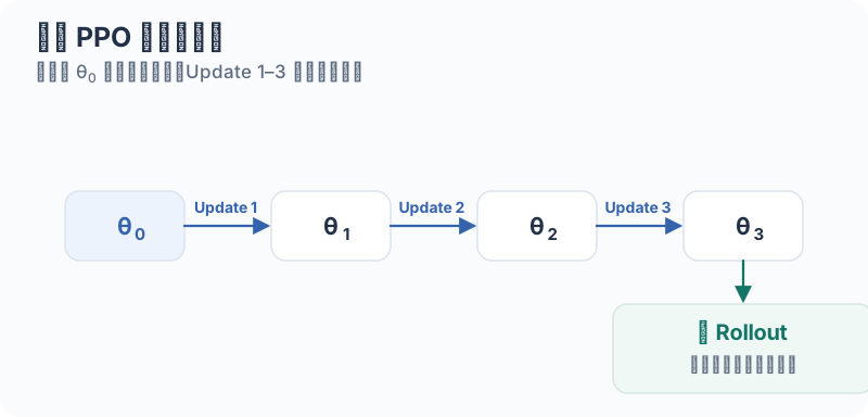
The denominator always stays the $\pi_{\theta_0}$ from sampling time, so from the second update onward $r\ne1$ already, because the parameters have been updated once. Clipping then prevents stale samples from continuously pushing the policy too far off.

Here $\theta_0$ is the snapshot of the model parameters at sampling time, and $\theta_1,\theta_2,\theta_3$ are the parameters after subsequent optimizer updates. Even when the numerator becomes $\pi_{\theta_2}$, the denominator should remain $\pi_{\theta_0}$ — otherwise the ratio no longer measures “how much the current policy has changed relative to the policy that generated these samples”.

But if we guarantee strict synchronization, train–inference consistency, and a single update per batch, then before the update $r_t(\theta_0)=1$ and clipping does nothing. Yet the gradient is not zero:

$$\left.\nabla_\theta r_t(\theta)\right|_{\theta_0} =\nabla_\theta\log\pi_{\theta_0}(y_t\mid h_t),$$

so:

$$\left.\nabla_\theta L_t^{\mathrm{CLIP}}\right|_{\theta_0} =A_t\nabla_\theta\log\pi_{\theta_0}(y_t\mid h_t).$$

Here the subscript $\left.\cdot\right|_{\theta_0}$ means: first differentiate with respect to the parameters, then substitute the sampling-time $\theta_0$. Although the value of $r_t$ is 1 here, its derivative with respect to $\theta$ is not zero — the right-hand side still carries $A_t$ times the logprob gradient. So the first single-step update’s gradient is locally equivalent to the advantage-weighted policy gradient.

After GRPO: What Are DAPO, Dr.GRPO, and GSPO Changing?

Having read about GRPO and PPO clipping, and then looking at the wave of papers that appeared after 2025 — DAPO, Dr.GRPO, GSPO and friends — we can understand them from the angle of “which GRPO pain point does each one solve”. Assembling the components from the previous sections, the complete objective GRPO actually optimizes is:

$$J_{\mathrm{GRPO}}=\frac1G\sum_{i=1}^{G}\frac1{T_i}\sum_{t=1}^{T_i}\ell_{i,t}, \qquad \ell_{i,t}=\min\big(r_{i,t}A_i,\ \operatorname{clip}(r_{i,t},1-\epsilon,1+\epsilon)A_i\big),$$

where $G$ is the group size, $T_i$ is the number of tokens in the $i$-th sample, $A_i=(R_i-\bar R)/(\sigma_R+\epsilon)$ is the within-group relative advantage, and $r_{i,t}=\pi_\theta(y_t\mid h_t)/\pi_{\mathrm{old}}(y_t\mid h_t)$ is the per-token new/old policy ratio. Thinking carefully through this formula term by term, there are four hidden hazards:

• The symmetric clip range $[1-\epsilon,1+\epsilon]$: the exploration space collapses too early. When a rare-but-correct reasoning path gets reinforced by a positive advantage, token probabilities rise quickly, $r_{i,t}$ soon hits the $1+\epsilon$ ceiling and the gradient zeroes out — the model’s newly explored ability gets braked prematurely, and the policy tends to concentrate on a few fixed routines.
• The numerator $R_i-\bar R$ of $A_i$: all-correct / all-wrong groups carry no signal. When all rewards in a group are identical, $\sigma_R=0$ and all $A_i=0$; the compute burned on that group of rollouts produces zero gradient — training is wasted.
• The $\frac1{T_i}$ in the reduction (and $\sigma_R$): unbalanced gradient weights. Each token of a long answer is diluted by its own length, while each token of a short answer gets amplified; dividing by $\sigma_R$ also quietly changes the relative weights of problems of different difficulty.
• The per-token $r_{i,t}$: violent noise in token-level probability ratios on long sequences. Single-step ratios have high variance and lack sequence-level coordination.

The various changes in DAPO, Dr.GRPO, and GSPO land precisely on these four spots.

DAPO: Clip-Higher

Recall PPO from earlier: the clipping range $[1-\epsilon, 1+\epsilon]$ is symmetric (e.g., uniformly $\epsilon=0.2$). DAPO’s first change splits this symmetric range into two independent bounds $\epsilon_{\mathrm{low}}$ and $\epsilon_{\mathrm{high}}$:

$$L_{\mathrm{DAPO},t} =\min\left(r_tA_t,\operatorname{clip}(r_t,1-\epsilon_{\mathrm{low}},1+\epsilon_{\mathrm{high}})A_t\right).$$

Here $\epsilon_{\mathrm{low}}$ and $\epsilon_{\mathrm{high}}$ control how far the ratio $r_t$ may deviate from $1$ downward and upward, respectively. The two need not be equal: DAPO keeps $\epsilon_{\mathrm{low}}$ unchanged while raising only the upper bound $\epsilon_{\mathrm{high}}$ (the so-called Clip-Higher). Note this does not directly amplify the value of a positive advantage $A_t$; it merely postpones the moment when ”$A_t>0$ and $r_t$ rising” hits the ceiling and loses gradient.

A concrete example with $\epsilon_{\mathrm{low}}=0.2$ and $\epsilon_{\mathrm{high}}=0.28$:

• For a positive-advantage sample ($A=+1$) at $r=1.25$: traditional PPO’s ceiling is $1.2$, where the gradient is already zero; DAPO’s ceiling is relaxed to $1.28$, so the model can keep reinforcing this token.
• For a negative-advantage sample ($A=-1$) at $r=0.5$: both lower bounds are $0.8$, so both have already triggered the brake and stopped pushing it down further.

Why go easy on the positive direction? When a model works on a hard problem and finally explores a rare-but-correct reasoning path, that path often represents a newly budding capability (and such trajectories usually deviate more from what came before). If, just because its new/old probability ratio $r_t$ rises quickly, we cut the gradient off early at $1.2$ per the old rules, we waste an extremely precious learning signal. Relaxing the upper bound gives these uncommon correct paths more headroom to be scaled up, mitigating the policy’s premature concentration onto a few fixed routines (i.e., entropy collapse).

That said, two subtleties when understanding Clip-Higher:

• Clip-Higher does not amplify the positive initial gradient at $r=1$: it doesn’t multiply positive advantages by a larger coefficient; it merely widens the runway along which the positive gradient avoids truncation across subsequent updates.
• Relaxing the upper bound does not guarantee entropy rises: although raising the probability of rare high-quality paths can help diversity, if what keeps getting reinforced happens to be an already-dominant, high-probability correct path (note: a large $r$ only means a large deviation, not that the trajectory is necessarily rare — if $\pi_\theta(a\mid h)=0.6$ and $\pi_{\mathrm{old}}(a\mid h)=0.5$, $r$ is also 1.2), the distribution actually sharpens and entropy falls. Moreover, a long correct answer often contains redundant steps, and a trajectory-level positive advantage reinforces that filler along with the rest.

DAPO: Dynamic Sampling

Earlier, when discussing GRPO’s advantage, we mentioned a situation: if all $G$ answers sampled for the same prompt are correct, or all wrong, the within-group standard deviation is $\sigma_R=0$ and the centered numerators $R_i-\bar R$ are all $0$ — the entire group produces no policy-gradient signal.

We can work out a simple probability exercise: for a given problem, assume each sample is independent with per-sample success probability $p$, and each group has $G$ samples. Then the probability that a group has “at least one correct and at least one wrong” (i.e., can produce a valid gradient) is:

$$\boxed{P(\mathrm{useful\ group})=1-p^G-(1-p)^G.}$$

Setting $G=8$ and plotting $P(\mathrm{useful\ group})$ against $p$: when the problem is too hard ($p\to0$) or too easy ($p\to1$), the vast majority of groups are all-wrong or all-correct; only problems of moderate difficulty most easily produce valid signal:

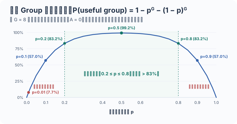
What DAPO’s Dynamic Sampling does is very direct: while collecting a training batch, it filters out these all-correct or all-wrong, zero-reward-variance groups and has the inference engine keep sampling new problems until the target number of valid groups is reached before starting a training update. This effectively allocates the training-step budget entirely to problems the current model can “reach with a small jump” — where it sometimes answers correctly and sometimes wrongly. As the model improves, the once-all-wrong hard problems see their $p$ gradually rise and naturally enter the valid range, forming an implicit difficulty scheduler: the problem distribution naturally starts easy, and later the easy problems thin out while the hard ones thicken.

But we should also be clear about its limits and costs:

• It is not an explicit easy-to-hard scheduler: if a super-hard problem stays at $p=0$ for the current model (always all-wrong), it gets filtered out forever and the model never learns it. For such problems you usually also need difficulty-adaptive sampling, process rewards (partial reward), task decomposition, or intermediate bridge tasks.
• Improved sample efficiency ≠ saved rollout compute: this is the most crucial point from a systems perspective. Suppose only $10\%$ of groups in the current problem bank are valid; to collect 128 valid groups for training, the inference side needs to sample about 1280 groups in expectation; at 8 answers per group, that’s a full 10,240 answer generations instead of the usual 1024. Sample efficiency per training step improved, but inference-side GPU compute may multiply — we only achieved “higher sample efficiency at the same step count”, not “higher efficiency at the same time budget”.

DAPO: Loss Reduction

In RL, what you divide by first and what you divide by afterward in loss reduction directly changes how much say answers of different lengths have in the total gradient. Revisit the reduction in $J_{\mathrm{GRPO}}$ from the beginning, $\frac1G\sum_{i=1}^{G}\frac1{T_i}\sum_{t=1}^{T_i}$: $G$ is the number of answers, and $T_i$ is the number of actually generated valid tokens in the $i$-th answer (excluding prompt and padding). This response-level reduction, common in vanilla GRPO, averages in two steps: first $\frac1{T_i}\sum_t$ compresses each answer into one mean; then $\frac1G\sum_i$ puts every answer on equal footing.

What are the consequences? Suppose a $G=2$ group has two answers: answer A is very concise, only 100 tokens; answer B is extremely verbose, 10,000 tokens. In $J_{\mathrm{GRPO}}$, each token of answer A carries a coefficient of $\frac{1}{2\times 100}=\frac{1}{200}$, while each token of answer B carries $\frac{1}{2\times 10000}=\frac{1}{20000}$. That is, a single token in short answer A has 100× the normalized weight of one in long answer B, even though the two answers have the same total normalized weight as wholes.

To eliminate this “per-token weight dilution by answer length”, DAPO switches to a token-level reduction closer to pretraining:

$$J_{\mathrm{DAPO}}=\frac{\sum_i\sum_{t=1}^{T_i}\ell_{i,t}}{\sum_iT_i}.$$

The denominator is no longer the number of answers $G$ but the total number of valid generated tokens in the entire batch, $N_{\mathrm{tokens}}=\sum_iT_i$. In other words, DAPO pours all tokens from all answers into one big pool and lets every token share the weight equally.

Now every valid token in A and B has exactly equal weight; but the cost is that answer B, at 10,000 tokens, contributes 100× the total trajectory weight of short answer A. It’s tempting to draw the crude conclusion: “GRPO favors short answers, DAPO favors long ones.” It’s really not that simple: advantages come in both signs, and the weighting acts on good and bad trajectories alike:

• Under GRPO (response-level), if the model produces a long-winded wrong answer ($A<0$, large $T_i$), dividing by the huge $T_i$ severely dilutes the punishment on each wrong token inside. The result: being wrong isn’t scary — just write long enough, and each bad token gets a light slap — which can actually make wrong answers grow ever more verbose during training.
• Conversely, under DAPO (token-level), if the model produces a very long answer that is ultimately correct but stuffed with filler in the middle ($A>0$), that long answer dominates the batch’s total gradient — which equally risks encouraging redundancy.

Also, from a cross-batch perspective: if two batches have 8K and 64K total valid tokens respectively, DAPO — dividing each by its own $\sum_i T_i$ — keeps the total gradient scale stable as long as the average per-token gradient vectors of the two batches are roughly similar; it won’t spontaneously scale up 8× just because one batch produced more characters (of course, real gradients also cancel out across dimensions; this is only about magnitudes).

DAPO: Overlong Reward Shaping

In long-chain-of-thought training, a common situation: the model is actually on the right reasoning track and the derivation is valuable, but by thinking so meticulously it slams into max_tokens and gets forcibly truncated before writing the final answer. Scoring it a flat 0 — or even a heavy penalty — just because no final answer can be extracted is needlessly brutal feedback.

To smooth out this reward cliff caused by hard truncation, DAPO introduces a smooth overlong punishment (Overlong Reward Shaping). For example, the original paper set up a buffer zone from 16,384 to 20,480 (a width of 4096 tokens) before the 20,480 cap:

$$R_{\mathrm{len}}(T)= \begin{cases} 0,& T\le 16384,\\ -\dfrac{T-16384}{4096},&16384<T\le20480,\\ -1,&T>20480. \end{cases}$$

Here $T$ is the number of generated tokens and $R_{\mathrm{len}}(T)$ is an additive length penalty (never positive): no penalty at all within 16,384; inside the buffer, the penalty grows linearly with length (e.g., at the buffer midpoint 18,432, the added penalty is $-0.5$); beyond 20,480 it is capped at $-1$. This penalty is added directly onto the task’s own correctness reward, rather than setting up a separate new policy loss.

Note that the purpose of Overlong Shaping is not to indiscriminately suppress long reasoning, but to keep the model from hitting a cliff-edge reward jump the moment it crosses the maximum-length red line. As for the specific numbers 16,384 and 20,480, they’re just one hyperparameter recipe from the original paper’s experiments; in practice you should adjust them to your own task’s length cap.

Dr.GRPO: Removing the Normalizations

If DAPO adds engineering and sampling strategy, Dr.GRPO’s core claim is subtraction: remove as many artificially introduced normalization terms as possible, restoring an objective closest to the unbiased policy gradient.

It makes two cuts to standard GRPO. The first removes the within-group standard deviation $\sigma_R$ from the advantage denominator, keeping only the mean subtraction (centering):

$$A_i^{\mathrm{Dr.GRPO}}=R_i-\bar R.$$

The second cut removes the dynamic denominator that depends on current sampled lengths in the loss reduction (whether each answer’s own $T_i$ or the current batch’s total length $\sum_i T_i$), replacing it uniformly with a fixed constant independent of how long the generations actually are (e.g., $G L_{\max}$):

$$J_{\mathrm{Dr.GRPO}}=\frac{1}{G L_{\max}}\sum_i\sum_t\ell_{i,t}.$$

Here $L_{\max}$ is a preset maximum generation length cap (or another fixed length constant) — not to be confused with the surrogate objective $L_t^{\mathrm{CLIP}}$ from earlier. For a given training configuration, $G L_{\max}$ is a thoroughgoing constant, while the numerator only sums over actually generated valid tokens.

Why remove the std? Compare two binary-reward (1 for correct, 0 for wrong) groups with $G=8$:

• Hard problem A: only 1 of 8 answers correct. Mean $\bar R=1/8$, population standard deviation $\sigma=\sqrt{7}/8$. Plugged into the standard GRPO formula, that single correct answer gets an advantage of $+\sqrt{7}\approx+2.646$, while the other, wrong answers get $-1/\sqrt{7}\approx-0.378$.
• Medium problem B: 4 of 8 answers correct. Mean $\bar R=1/2$, standard deviation $\sigma=1/2$. The correct and wrong answers’ advantages are a mild $+1$ and $-1$.

Because of dividing by $\sigma_R$, standard GRPO gives rare successes enormous positive weight on hard problems ($p$ near 0); symmetrically, on very easy problems ($p$ near 1) it also heavily punishes rare failures. Algebraically, as long as a group is not all-correct or all-wrong, normalizing by the population standard deviation makes the sum of squared advantages within the group constant, $\sum_i A_i^2 = G$ — that is, no matter what difficulty range a problem is in, the overall magnitude of the gradient it produces is forcibly equalized.

What if we remove $\sigma_R$, as Dr.GRPO does? The sum of squares for binary rewards becomes $\sum_i A_i^2 = Gp(1-p)$: the hard problem A group above yields 0.875, while the medium problem B group yields 2, so the weight naturally tilts toward medium-difficulty problems. A minimal toy model shows why this is the “raw” gradient scale: suppose the model has a single learnable scalar logit $z$ controlling the probability of the “answer correctly” action, $p=\sigma(z)=\frac{1}{1+e^{-z}}$ ($\sigma(\cdot)$ being the sigmoid), so the expected reward is $J(z)=p$. Its true derivative with respect to $z$ is exactly:

$$\frac{\partial J}{\partial z}=p(1-p).$$

(Here $\partial J/\partial z$ is the partial derivative with respect to the scalar $z$, consistent in direction with the earlier $\nabla_\theta J$ for the whole parameter vector.) If we forcibly divide by $\sigma_R=\sqrt{p(1-p)}$ when estimating the gradient, the expected gradient’s scale gets distorted from $p(1-p)$ to roughly $\sqrt{p(1-p)}$, artificially changing the relative weights of problems at different difficulty levels — this is the question-level difficulty bias that Dr.GRPO criticizes. Of course, this is only a simplified model for conveying intuition; sample standard deviations under finite sampling, and gradient vectors of real deep networks, are far more complicated.

Personally, though, I don’t think “giving rare successes on hard problems higher weight” is necessarily a bad thing. If your training goal is to push the capability frontier, a lucky success on a hard problem is priceless to begin with. The issue is not whether to weight, but that the weighting should be a conscious choice, not something silently done for us by the $\sigma_R$ in the denominator as a side effect of applying the formula. We can even unify the two choices into a single spectrum with a hyperparameter $\alpha$:

$$A_i^{(\alpha)}=\frac{R_i-\bar R}{(\sigma_R+\epsilon)^\alpha},\quad 0\le\alpha\le1.$$

Here $\alpha$ is a knob for manually tuning the normalization strength: $\alpha=0$ degenerates to Dr.GRPO, $\alpha=1$ is standard GRPO, and values in $(0,1)$ are compromises. (To be clear, this formula is only meant to help you see the design space; it is not a new algorithm validated at scale. And for extremely hard problems where $p\approx0$ and no correct answer can ever be sampled, no amount of $\alpha$ helps.)

Likewise, Dr.GRPO’s switch to the fixed denominator $G L_{\max}$ is not free: if batch B has 8× the valid generated tokens of batch A, with similar average per-token gradient direction, then under the fixed denominator $G L_{\max}$, batch B’s overall gradient is 8× batch A’s; whereas DAPO’s dynamic denominator $\sum_i T_i$ keeps the two batches’ gradient scales close. So these are fundamentally different choices about weight allocation across sample lengths and the effective learning-rate scale across batches — not a black-and-white right-or-wrong. So has Dr.GRPO (which they call “GRPO Done Right”) really been done right? Honestly, I’m not so sure either.

GSPO: Sequence Ratio

When we discussed importance sampling earlier, we left a thread hanging: theoretically, the importance ratio of an entire autoregressive trajectory should be the product of all token ratios $\prod_{t=1}^T r_t$; because that product necessarily explodes or vanishes on long sequences, PPO and GRPO compromised to having each position look only at its own single-step ratio:

$$r_t=\frac{\pi_\theta(y_t\mid h_t)}{\pi_{\mathrm{old}}(y_t\mid h_t)}.$$

But computing and clipping ratios independently per token brings new troubles on long sequences — especially in MoE model training: a single token’s probability ratio is very noisy; within one answer, some tokens get clipped and others don’t, which easily breaks the coordination of the whole sequence’s update.

So GSPO (Group Sequence Policy Optimization) proposes pulling the perspective back to the whole sequence — but instead of using the explosive product, it first takes the arithmetic mean of $\log r_t$ over all tokens of the answer, then exponentiates back:

$$\boxed{r_{\mathrm{GSPO}}=\exp\left(\frac1T\sum_{t=1}^{T}\log r_t\right).}$$

Unpacking it: because the average of logarithms equals the $T$-th root of the product, $r_{\mathrm{GSPO}}=\left(\prod_{t=1}^{T}r_t\right)^{1/T}$ — it is precisely the geometric mean of the probability ratios of all tokens in the answer. This way, no matter how long the answer, $r_{\mathrm{GSPO}}$ stays at the same numeric magnitude as a single-step ratio (a positive number near 1), and GSPO uses this sequence-level ratio to uniformly measure and clip the relative change of the whole answer. The original paper reports that this effectively reduces the noise of per-token ratios on long sequences and significantly improves RL training stability for the Qwen family (especially MoE models).

But note: the geometric-mean ratio $\left(\prod_t r_t\right)^{1/T}$ is mathematically absolutely not equal to the strict, unbiased full-trajectory importance ratio $\prod_t r_t$! Their variance properties and corresponding surrogate objectives are completely different — never mistake GSPO for “finally achieving strictly unbiased sequence-level importance sampling”.

Looking further along this line, 2025 saw plenty of interesting explorations: CISPO chooses to clip the importance weight itself, rather than the gradient of the whole PPO surrogate; VAPO chooses to return to the PPO route with a value/critic network, optimizing bias and variance specifically for long chains of thought. Also, in some implementations GSPO can reduce the reliance on recomputing per-token old-policy logprobs on the training side (depending on the training recipe). Together, these works demonstrate one thing: GRPO did not end RL algorithm design; people are still searching for better engineering trade-offs inside the “bias–variance–long-sequence stability” impossible trinity.

Synchronous and Asynchronous RL

Four Easily Confused Policies

When reading the code of an RL training framework, you’ll quickly discover that for “computing some policy’s logprobs”, there are four different variable names:

Name	Meaning	Where it’s used
$\pi_b$ / rollout_logprobs	The behavior policy that actually sampled the generated tokens	Importance weight denominator; train–inference consistency monitoring
$\pi_{\mathrm{old}}$ / old_logprobs	The old-policy baseline for this round of PPO updates (often recomputed by the training engine)	Denominator of the PPO / GRPO ratio
$\pi_\theta$ / current_logprobs	The current training policy being forward- and back-propagated	Numerator of the PPO / GRPO ratio
$\pi_{\mathrm{ref}}$ / ref_logprobs	The frozen reference policy (usually the initial RL model)	Reference KL provides a metric of “how far we’ve drifted from the start”

The subscripts alone reveal their identities: $b$ stands for behavior (the policy that actually sampled the data in the inference engine), $\mathrm{old}$ is the comparison baseline fixed for this PPO optimization cycle, $\theta$ is the parameters currently being updated by the optimizer, and $\mathrm{ref}$ is the reference model serving as the anchor. Of course, they all have exactly the same architecture — apart from $\pi_{\mathrm{ref}}$, the others are often just weight snapshots from different moments, or the same weights computed by different engines (inference vs. training); you don’t actually need to fit four models into GPU memory simultaneously.

The two things we chiefly need to pin down are: are these two probabilities computed with the same version of the model weights? and are they computed on the same kernels? Without clarity on these two, you’ll misattribute the various “KL”s in training logs: Reference KL (comparing $\pi_\theta$ vs. $\pi_{\mathrm{ref}}$), PPO KL (comparing $\pi_\theta$ vs. $\pi_{\mathrm{old}}$), and Train–Inference KL (same weights, comparing training-engine vs. inference-engine outputs) may all be labeled kl in the logs, but they measure three completely different pairs of distributions.

Synchronous RL

Many people intuitively assume: as long as I run strictly synchronous RL — i.e., honestly wait for a whole batch of data to finish generating before training — then the training-time probability ratio $r_t$ should equal 1.

Not so. As mentioned earlier with PPO, the standard PPO design allows multiple epochs or minibatch updates on the same batch of rollout data. As soon as the first gradient update moves the parameters from $\theta_0$ to $\theta_1$, from the second update onward you’re already in the off-policy state of “sampled by old policy $\theta_0$, trained with new policy $\theta_1$”, and PPO clipping immediately starts working. What’s even more likely, though, is that due to train–inference inconsistency (non-associativity of floating-point arithmetic), the rollout policy and the policy computed by the training forward pass disagree, making $r_t$ differ from 1.

In other words, only when all three stricter conditions hold — identical weight versions, numerically identical train–inference computation, and a single optimizer update per batch — is the ratio at gradient-computation time strictly 1. And as we’re about to see, even if you satisfy all three, engineering implementations still have other pitfalls waiting for you.

The Gains and Costs of Fully Async

Why is everyone racing into async RL now? Because rollouts in long-chain-of-thought and agent settings suffer from severe long-tail effects. In synchronous mode, if you want to collect 1024 trajectories before training, and even a small handful of problems generate 256K-token or even 1M-token responses, or a few code sandboxes hang, the entire cluster’s GPUs must sit idle waiting for those few slow samples — utilization is terrible.

The core idea of an asynchronous system is to split rollout, reward/verifier judging, training, and weight synchronization into a pipeline, letting each stage run at its own pace without idling each other:

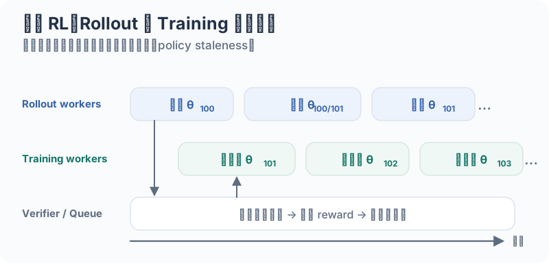
This significantly raises GPU utilization and shortens end-to-end training time, but there’s no free lunch — it necessarily introduces policy staleness: in the figure, a sample generated by the old weights $\theta_{100}$ may sit in a queue, and by the time the training side actually consumes it, the training-side weights may have already advanced all the way to $\theta_{103}$. More extreme: if the system allows hot-swapping inference weights mid-generation, then the first and second halves of a single trajectory can even be stitched together from different model versions! At that point, if you still want importance sampling to be correct, you must record the true behavior policy at token granularity — and even whether the KV cache left behind by the old weights in the first half can be reused by the new weights becomes semantically questionable.

From a scheduling-paradigm view, mainstream designs today roughly fall into three tiers: Synchronous (generate a batch, then train a batch), Pipelined (separate rollout/training GPU pools, pipeline overlap at batch granularity), and Fully Async (inference side generates continuously, training side consumes continuously, version lag managed explicitly). Incidentally, “whether rollout and training are deployed on separate GPUs (disaggregated vs. colocated)” and “whether scheduling is sync or async” are two independent matters — real systems can combine them freely.

Numerical Mismatch vs. Policy Staleness

With all that covered, we can finally decompose “why RL training goes off-policy” into two orthogonal root causes. For the same sampled token $y_t$ under a fixed prefix $h_t$, let’s define three probability values:

$$\begin{aligned} p_b &=\pi^{\mathrm{rollout}}_{\theta_b}(y_t\mid h_t),\\ p_o &=\pi^{\mathrm{train}}_{\theta_b}(y_t\mid h_t),\\ p_c &=\pi^{\mathrm{train}}_{\theta_c}(y_t\mid h_t). \end{aligned}$$

How to read these three? The superscripts and subscripts suffice: the superscripts $\mathrm{rollout}$ and $\mathrm{train}$ distinguish which engine does the computation (e.g., SGLang/vLLM vs. Megatron/FSDP), while the subscripts $\theta_b$ and $\theta_c$ distinguish which version of the model weights is used ($\theta_b$ is the behavior weights that generated this data; $\theta_c$ is the current weights now consuming it in training). So $p_b$ is the true probability computed by the inference engine at sampling time, $p_o$ is the probability recomputed by taking those same old weights $\theta_b$ into the training engine, and $p_c$ is the probability computed by the new weights $\theta_c$ in the training engine. Note that all three numbers always evaluate the conditional probability of the same already-sampled token $y_t$ in the same context — they are three scalars, not three re-samplings.

With these three definitions, everything snaps into focus:

• Even when inference and training use exactly the same weights $\theta_b$, differences in underlying kernels, quantization precision, floating-point rounding order, attention implementations, or MoE routing can make $p_b\ne p_o$. This deviation, purely from different software/hardware execution paths, is numerical mismatch (train–inference numerical inconsistency);
• Meanwhile, within the same training engine, $p_o\ne p_c$ caused by the weights having advanced from $\theta_b$ to $\theta_c$ is pure policy staleness.

So the total probability ratio of the current training policy relative to the true sampling policy, $\frac{p_c}{p_b}$, decomposes cleanly into a product of two terms:

$$\boxed{\frac{p_c}{p_b}=\underbrace{\frac{p_o}{p_b}}_{r_{\mathrm{num}}}\cdot\underbrace{\frac{p_c}{p_o}}_{r_{\mathrm{stale}}}.}$$

Here $r_{\mathrm{num}}$ specifically measures same weights, across engines numerical deviation, while $r_{\mathrm{stale}}$ specifically measures same engine, across versions policy drift. Taking logarithms on both sides turns the product into a sum:

$$\log\frac{p_c}{p_b}=\left(\log p_o-\log p_b\right)+\left(\log p_c-\log p_o\right).$$

But here’s a mathematical subtlety: what gets added are signed logprob differences, not absolute values! By the triangle inequality, $|\Delta_{\mathrm{num}}+\Delta_{\mathrm{stale}}|$ generally does not equal $|\Delta_{\mathrm{num}}|+|\Delta_{\mathrm{stale}}|$. When analyzing experiment logs, we must never crudely subtract “the mean absolute error of sync training” from “the mean absolute error of async training” to back out how large staleness is.

With this decomposition understood, we can put the two in their proper places: in async training, staleness is the inevitable price of pursuing throughput, but same-weights numerical mismatch is noise that engineering can eliminate. Only by first getting numerical consistency right at the lowest layer do we obtain a clean, accurate old-policy baseline (making $p_o = p_b$), and only then can we hand the true version lag over to upper-layer algorithms like TIS / MIS to correct (we’ll get there shortly); conversely, even if you achieve perfect bitwise consistency, it won’t eliminate the $r_{\mathrm{stale}}$ that async training brings.

A Concrete Example

You might think: “So what if training and inference compute slightly different probabilities? Close enough is fine, right?” Let’s work out a very concrete example.

Suppose we’re running strictly synchronous RL; the model weights are still the initial $\theta_0$, not updated a single step. But due to train–inference inconsistency, the rollout engine and the training engine disagree on the probabilities of two particular tokens. If we directly use the rollout-recorded rollout_logprobs as the PPO ratio denominator:

Token	Rollout Engine ($p_b$)	Training Engine ($p_o$)
Correct Token ($A=+1$)	0.4	0.6
Wrong Token ($A=-1$)	0.6	0.4

Let the good token’s advantage be $A_{\mathrm{correct}}=+1$ and the bad token’s $A_{\mathrm{wrong}}=-1$, with PPO’s clip range at the standard $[0.8, 1.2]$. Computing the clipped surrogate objective for the first training step:

• Correct Token: ratio $r = 0.6 / 0.4 = 1.5$, so $L = \min(1.5 \times 1,\ 1.2 \times 1) = 1.2$ — clipped, gradient zeroed!
• Wrong Token: ratio $r = 0.4 / 0.6 \approx 0.667$, so $L = \min(0.667 \times (-1),\ 0.8 \times (-1)) = -0.8$ — clipped, gradient zeroed too!

The model hasn’t done a single gradient update yet, and purely because the two engines’ computed probabilities disagree, both tokens trip PPO’s clip at the very first step, completely losing their learning signal! Now what if async training is layered on top? Suppose $p_b=0.40,\ p_o=0.60,\ p_c=0.66$:

$$r_{\mathrm{num}}=\frac{0.60}{0.40}=1.5,\qquad r_{\mathrm{stale}}=\frac{0.66}{0.60}=1.1,\qquad r_{\mathrm{total}}=\frac{0.66}{0.40}=1.65.$$

See — the true policy staleness is only a mild $r_{\mathrm{stale}}=1.1$, well within $[0.8, 1.2]$, which should never have been truncated; it’s purely because of the $1.5$ numerical deviation multiplied in front that it got unfairly clipped.

In engineering practice there’s also a more insidious, head-in-the-sand approach: some frameworks, at the start of training, run a forward pass with the training engine to recompute old_logprobs (i.e., $p_o$) and use that as the PPO denominator. Now the ratio PPO sees becomes $p_c / p_o = 1.1$, and the ppo_kl and clipfrac in the TensorBoard logs look serene and perfectly healthy. But in reality? The true sampling ratio is $p_c / p_b = 1.65$! This approach doesn’t eliminate the deviation; it merely hides the true sampling-distribution deviation outside the PPO ratio’s field of monitoring view. Even in “strict sync + one update per batch”, as long as the training side uses its own recomputed $p_o$ as the denominator, the ratio superficially stays at $1$ while under the hood the model is still optimizing against something other than the distribution that actually produced these samples.

One more step along this decomposition: since $r_{\mathrm{total}} = r_{\mathrm{num}} \cdot r_{\mathrm{stale}}$, what if some token happens to hit $r_{\mathrm{num}}=1.5$ while also, due to version lag, $r_{\mathrm{stale}}=0.7$?

Multiply them and the total ratio is $r_{\mathrm{total}} = 1.05$! If you only watch the final combined Total Ratio on your dashboard, you’d conclude that training and sampling policies are highly consistent (only 5% apart); yet in reality, both the underlying numerical deviation and the version lag are way off — they just happen to cancel, one positive and one negative. This is why, when diagnosing an RL system, you must log the same-version train–inference numerical difference, the policy version-lag steps, and the new/old policy drift separately — never blindly knead them into a single average and call it a day.

TIS and MIS

Since train–inference deviation and async lag can hardly be driven to zero in real systems, what can we do about it at the algorithm level?

The most common remedies today are TIS (Truncated Importance Sampling) and MIS (Masked / Filtered Importance Sampling).

• TIS is direct: since $\pi_b$ actually generated the samples, explicitly compute the training policy’s ratio relative to the true sampling policy, $w_t = \pi_{\mathrm{train}}(y_t\mid h_t) / \pi_b(y_t\mid h_t)$, and multiply it onto the $t$-th token’s gradient as an importance weight; to keep outlier $w_t$ values from blowing up gradient variance, also give $w_t$ a truncation cap — in essence, introducing a little truncation bias in exchange for stable variance.
• MIS is more blunt: if a sample’s or token’s deviation exceeds a threshold, just mask it (filter it out) so it doesn’t participate in the gradient update. In async agentic RL systems, people further combine trajectory-level trust regions, staleness limits, and stale-sample dropping.

When reading code or logs, be careful to distinguish TIS’s weight $w_t$ from the PPO ratio discussed earlier: when constructing $w_t$, the denominator $\pi_b$ must be the probability the inference engine actually assigned that token at generation time; $w_t > 1$ means the current training policy considers the token more likely than at sampling time, so its weight gets scaled up, while $w_t < 1$ means scaled down. Moreover, TIS’s truncation (capping the weight $w_t$ directly to suppress variance) and PPO’s clipping (a one-way brake on the surrogate objective keyed to the advantage’s sign) are two entirely different things — never conflate tis_clipfrac and pg_clipfrac in the logs.

Hence what modern RL infrastructure advocates is letting each layer solve only its own problems:

1. Numerics and operators: eliminate same-weights numerical mismatch between the training and inference engines as much as possible;
2. System scheduling: control the async pipeline’s version staleness and accurately record each token’s version;
3. Algorithm: use TIS / MIS and PPO clipping as backstops, controlling the bias and variance of off-policy updates;

The Broader Systems Landscape and Agentic RL

If we lift our gaze from a single loss formula to the whole 2025–2026 evolution of LLM RL infra, the core directions everyone is pushing on are clear: asynchronous training frameworks (e.g., AReaL, Slime, SkyRL), speculative-decoding acceleration for long-chain-of-thought rollouts (e.g., introducing Speculative Decoding / MTP under the strict constraint of preserving the sampling distribution losslessly), train–inference routing consistency for MoE models (e.g., R3, Rollout Routing Replay), and multi-turn tool use and agentic RL.

A few representative engineering numbers (these speedups depend heavily on the specific model scale, hardware, and workload): AReaL, in its 2025 paper’s experimental setup, achieved up to about 2.57× training throughput over a synchronous system (though my experience using AReaL last year was really quite bad); NVIDIA NeMo RL’s 2026 speculative-decoding work achieved 1.5–1.8× rollout throughput gains on a specific 8B reasoning-model configuration, and sped up synchronous end-to-end RL training by up to 1.4×.

In agentic RL settings, even the shape of the training data itself changes qualitatively. In traditional math-problem or single-turn dialogue RL, one data point is simply Prompt → Response → Reward; but in agent tasks, a trajectory becomes a multi-turn interaction chain:

$\text{State}\to\text{Action}\to\text{Observation}\to\dots\to\text{Reward}.$

Here State is the current external environment and context, Action is a reasoning segment the model generates or a tool-call instruction it issues, Observation is the real result returned by the external tool, code interpreter, or sandbox after execution — and so on for many rounds ($\dots$), until the task ends and the verifier issues a final (or per-step) Reward. For example, a coding agent fixing a bug might first read a file, run a shell command, glance at the error log, then modify the code and rerun the unit tests.

This shape throws a whole new set of engineering problems at the underlying system:

• Credit assignment: if an agent makes 30 tool calls in a row and the last step fails on a timeout with a score of 0, were all 29 prior investigation steps also wrong?
• Environment determinism and resource bottlenecks: how do you keep code sandboxes and external environments reproducible? When thousands of sandboxes run tests concurrently, the bottleneck often shifts from GPUs to CPU, network I/O, and long-tail sandbox scheduling.
• Extremely long trajectories: for agentic tasks, trajectory length grows from the 32K of traditional math tasks to 256K or even 1M. Rollout pressure becomes enormous, and left uncontrolled, it further amplifies staleness.

This again confirms the earlier point: judging an RL infra must never rely on static tokens/sec throughput, but on how much real capability improvement each GPU-hour buys. “GPU hours vs. performance gain” has in fact become the de facto optimization standard — for example the vLLM team’s “Finish RL Training Faster” that I’ll discuss later, and the recent article from the Tencent Hunyuan team here ↗.

A vLLM Case Study

Of the four-layer architecture mentioned in the last section, the foundation is “eliminating same-version train–inference mismatch at the numerical layer”. How is this layer actually implemented in engineering? An excellent case to dissect is the vLLM team’s 2026 post, Finish RL Training Faster — Bitwise-Consistent, High-Performance, Agent-Driven. To read the original, click here ↗.

Non-Associativity of Floating-Point Arithmetic

The starting point of all these problems is one of the most basic facts of computer science: floating-point addition is not associative.

$$(a+b)+c\ne a+(b+c).$$

Here’s an FP32 example you can verify at a glance: take $a=-2^{24},\ b=2^{24},\ c=1$. If you compute $(a+b)+c$ first, the positive and negative $2^{24}$ cancel to $0$, and adding $1$ gives $1$. But if you instead compute $b+c$ first, then — since FP32’s mantissa holds only 24 bits — the $1$ in $2^{24}+1$ gets rounded away for lack of precision ($16777217$ sits exactly halfway between $16777216$ and $16777218$, and rounds to the even mantissa, $16777216$), leaving $2^{24}$; finally adding $a=-2^{24}$ yields $0$!

And inside a matrix multiplication $Y=XW$, what the hardware does is precisely massive amounts of this kind of accumulation: if the input $X$ has shape $M\times K$ ($M$ is the number of token rows being processed) and the weights $W$ are $K\times N$ ($N$ is the output feature dimension), then every element of the output matrix $Y$ (shape $M\times N$) is a length-$K$ inner-product sum $Y_{m,n}=\sum_{k=1}^{K}X_{m,k}W_{k,n}$. This means: even if two kernels are fed exactly the same FP8 inputs, use exactly the same weights, and even accumulate internally in high-precision FP32 registers — as long as they add these $K$ terms in a slightly different order, the resulting floats can differ in the last few bits (ULPs, units in the last place).

In ordinary inference serving, a few ULPs of difference in the last place are harmless. But in RL training, these computed logprobs get divided into importance ratios; worse, modern LLMs are full of discrete choices like MoE top-K routing and top-K sparse-attention indices (e.g., DSA, CSA, CSA v2, etc.) — the moment a value sits right at a ranking tie point, the selected experts or attention positions can swap out entirely, and the downstream difference is amplified instantly.

Bitwise Consistency

For this reason, the vLLM team’s post decomposes “true bitwise train–inference consistency” into five progressively stacked requirements:

1. Kernel determinism: the same kernel, fed identical inputs, must produce identical outputs no matter how many times it runs.
2. Batch invariance: a request’s result must never change depending on who else is co-batched with it, or how many requests there are.
3. Stage consistency: the same token must produce identical results whether it goes through the Prefill path or the Decode path.
4. Distributed consistency: the reduction order of cross-GPU communication, or changes in parallelism schemes like TP / EP / CP, must not affect the numerical results on the compared paths.
5. A shared numerical contract: quantization scheme, rounding rules, intermediate computation precision, operator tiling, tie-breaking in discrete rankings, and reduction merge order must all align between the training and inference sides.

Bitwise consistency means: before every parameter update, with a fixed weight version and the same token prefix, subtracting the training-side recomputed old_logprob from the rollout_logprob recorded by the inference engine at sampling time must yield exactly 0 — not the traditional “error below $10^{-5}$ counts as aligned”. (Of course, after a minibatch update changes the weights, the policy itself has changed, which naturally falls outside this definition.)

You can see these five requirements interlock, none substitutable for another: a single operator being deterministic doesn’t mean results stay the same across batch sizes; achieving batch invariance doesn’t mean prefill, decode, and the training forward align; and even a bitwise-identical forward pass certainly doesn’t mean the backpropagation gradients are automatically exact.

Batch Invariance

In vLLM’s original default implementation, small batches with $M<32$ dispatch to the latency-optimized FlashInfer kernel, while larger batches switch to the throughput-oriented DeepGEMM; beyond that, the MoE router, small matrix multiplies, and mHC splitting each have their own shape-based dynamic branches (heuristics). Under inference’s continuous batching, how many requests are co-batched with a given request changes at every decode step; during training, meanwhile, we habitually pack all sequences into one giant packed batch for a single forward pass, which is usually fixed. The result: the same token doesn’t even run on the same GEMM kernel at inference and training time, so of course the accumulation orders differ wildly.

The vLLM team’s fix: forcibly enable DeepGEMM’s batch-invariant mode, fixing the accumulation tiling of each row’s inner product; unify the router to a fixed FP32-output GEMM; fix the reduction strategy for small matrices; and pin mHC’s split to 1. The costs: some inference-latency optimization at very small batch sizes is sacrificed, and the training side must re-quantize the master weights at every forward pass.

Stage Consistency

With matrix multiplication settled, next comes attention. Though the attention formula on paper is forever one thing:

$$O=\operatorname{softmax}(QK^\top/\sqrt d)V, \qquad o=\frac{\sum_j e^{s_j-m}v_j}{\sum_j e^{s_j-m}}.$$

(Notation refresher: on the left is the familiar matrix form, with $Q,K,V$ the Query, Key, and Value matrices and $d$ the per-head vector dimension; on the right we zoom into the output vector $o$ of one specific query, where $s_j=q^\top k_j/\sqrt d$ is its attention score against the $j$-th historical position, $m=\max_j s_j$ is the max subtracted to prevent exponential overflow, $e^{s_j-m}$ are the unnormalized weights, the numerator is the value-weighted sum, and the denominator normalizes.)

Simple as the formula looks, on GPUs FlashAttention internally uses tiled online softmax (if you don’t know how FlashAttention works, the TL;DR is: to avoid repeatedly reading and writing HBM during the softmax above, it uses an online algorithm). How the tiles are cut, whether split-KV parallel reduction happens, even which instruction approximates $\exp$ at the bottom — all of it directly affects the intermediate floating-point rounding. Worse, in inference engines the prefill stage processes many queries of a whole sequence in parallel, while the decode stage takes only the 1 newly generated query at a time to look up in the paged KV cache — in mainstream frameworks these two stages run on two entirely different kernels! So even if your KV cache storage itself is lossless, the same token’s output computed via prefill (corresponding to training’s whole-sequence parallel forward) and via decode (corresponding to inference’s token-by-token generation) still won’t match.

In DeepSeek-V4-Flash’s implementation this contradiction is especially acute: its prefill path first dequantizes the FP8 KV cache back to BF16, then calls the sparse-attention operator; while the decode path, to save bandwidth, directly calls a native FP8 FlashMLA kernel. To forcibly align these two paths, the vLLM consistency version makes decode give up the native FP8 operator too, uniformly switching to read from the FP8 cache → gather and dequantize into a temporary BF16 workspace → call exactly the same flash_mla_sparse_fwd operator as prefill.

The benefit is keeping the core memory savings of the FP8 KV cache (the post measures memory usage at roughly 57% of BF16 KV); the cost is an extra gather and dequantization step during decode. The training side must cooperate too: although the training forward is computed in one shot and needs no autoregressive KV cache at all, the training side still artificially allocates a private FP8 cache buffer, forcibly subjecting the training-time $K$ and $V$ to the exact same “quantize to FP8 then dequantize back to BF16” operation — solely to replicate inference’s rounding behavior.

But splicing the forward’s quantized operators onto the backward’s differentiation is a problem of its own: for the approximated tensor $\widetilde K=\operatorname{dequant}(\operatorname{quant}(K))$ that has been through “quantize then dequantize”, since quantization is a discrete staircase function, its Jacobian is zero almost everywhere — backpropagated gradients would simply die there. To pass gradients through, the post adopts the classic STE (Straight-Through Estimator) from quantization-aware training, directly approximating $\partial\widetilde K/\partial K\approx I$ in the backward pass — effectively pretending quantization and dequantization don’t exist and passing the upstream gradient to $K$ untouched. For a few fused operators that can’t be directly autodiffed, they built a separate parallel differentiable computation graph in PyTorch just for computing gradients, while the forward activations are replaced by the inference kernel’s outputs.

Distributed Consistency

At the MoE layer, train–inference inconsistency gets even trickier. First, the two sides organize expert-token layouts in memory completely differently. To make the same token compute bitwise-identical results under these two radically different memory layouts, three details must be pinned down simultaneously:

• The scaling factors and rounding rules must be identical when each input row undergoes FP8 dynamic quantization;
• The expert-layer DeepGEMM must run in batch-invariant mode, ensuring that one token row’s result is unaffected by which neighboring token rows sit above and below it;
• When the activation layer computes SiLU(gate) * up, the multiplication must be completed in one go in FP32 precision, with a single final rounding to BF16 — never rounding to BF16 once at the SiLU output and again after multiplying by up.

With single-GPU operators settled, cross-GPU communication reduction remains. In DeepSeek-V4-Flash’s experimental configuration, the rollout side uses EP8, while the training side uses EP32 + CP4. The two sides don’t even share parallelism degrees — how could they possibly compute bitwise-identical results? Their experimental findings and solution:

1. By not using TP at all, they avoid TP All-Reduce, the step most prone to introducing floating-point error through differing cross-GPU reduction orders;
2. Expert-parallel EP All-to-All communication only moves tokens intact to their target GPUs, with no cross-GPU additive reduction in between; after each expert finishes its output and All-to-All returns the token to its original GPU, the local GPU strictly performs the accumulation locally in FP32, in a fixed top-K order;
3. Context parallel (CP) here likewise only passes and concatenates KV state, with no cross-GPU summation that would change the compared results.

Running Two Minimal RL Experiments

With the systems intuition built above, let’s now look at real runs: what the staleness looks like, how big the numerical error is, and “what a healthy run looks like”. I ran two experiments with slime: the same Qwen3.5-0.8B doing GRPO on GSM8K — one sync, one async, 120 steps each.

Hyperparameter Setup

Shared configuration:

• Qwen3.5-0.8B / GSM8K / GRPO, Slime framework, temperature 1.0, 1024 responses rolled out per step; num_steps_per_rollout=1 (one optimizer update per batch of data); use_rollout_logprobs=false (the PPO ratio’s denominator doesn’t use the inference engine’s logprobs — the training engine recomputes them with the same-version weights); use_kl_loss=true but kl_loss_coef=0.0: the reference KL is computed but contributes no gradient.

Differing configuration:

• Sync run: single node, the same GPUs alternate between inference and training, per-response cap of 1024 tokens;
• Async run: also single node, 4 GPUs dedicated to rollout and 4 dedicated to training, response cap relaxed to 2048 tokens, and TIS enabled.

Note: these two runs are not a single-variable comparison. The async run’s length cap is higher than the sync run’s, so the async run’s higher reward later on is to be expected.

Reward, Eval

Reward first:

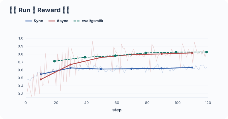
Overall, both runs’ rewards look healthy — trending up throughout, with no reward collapse.

• Sync’s reward gains are pronounced in the first 20 steps (0.54 → 0.63), then it sits on a 0.61–0.63 plateau for the remaining 100 steps. This is “fast learning early, diminishing marginal returns later” — not a collapse (a collapse would look like reward staying low so the model gets no reward signal, or reward declining). In fact, the eval results show continued climbing later on. That part can be explained as the payoff of the model’s pass@1 becoming more stable.
• Async’s reward climbs from 0.48 all the way to 0.82, with no plateau. But the scatter of the thin line shows the noise at a glance: the last 20 steps have a single-step standard deviation of 0.074 (Sync’s is only 0.021), oscillating between 0.63 and 0.95 per step. Rollout reward is noisy, which further argues for downstream eval tasks to track the model’s trajectory.

Entropy, KL

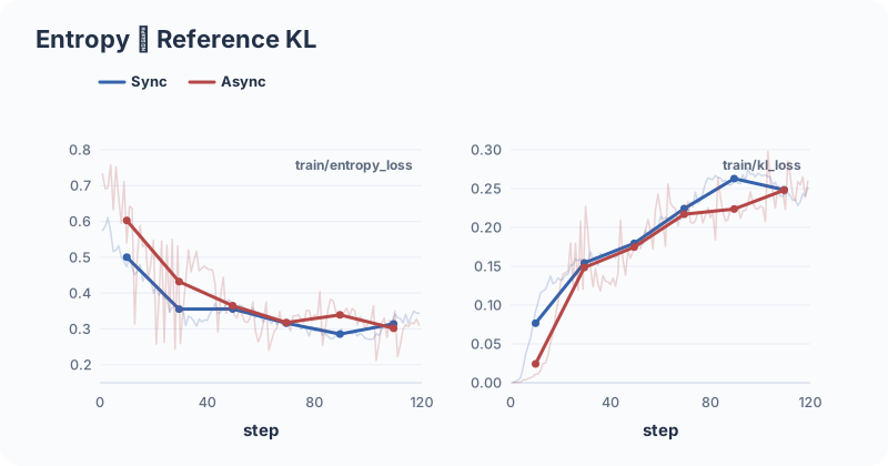
• Falling entropy is the model going from confused to confident about its reasoning steps — a normal decline. Judging entropy collapse requires reading several metrics together: if entropy cliffs toward zero, reward crashes in lockstep, and within-group solutions become carbon copies of one another, that’s probably a collapse.
• Reference KL slowly rises to 0.25 and then flattens. RL’s whole point is to deviate from the initial model, so a widening KL is inevitable; growth in reference KL is not much of a concern. (It does not indicate train–inference inconsistency!)

Length, Truncation

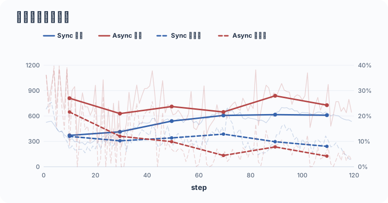
Both truncation rates converge. On GSM8K, hitting the length ceiling means the answer was never written and scores 0, so a high truncation rate is bad. But GSM8K is a very, very easy benchmark, so the current max length is a reasonable setting — by the end, the model mostly finishes its answers within the cap.

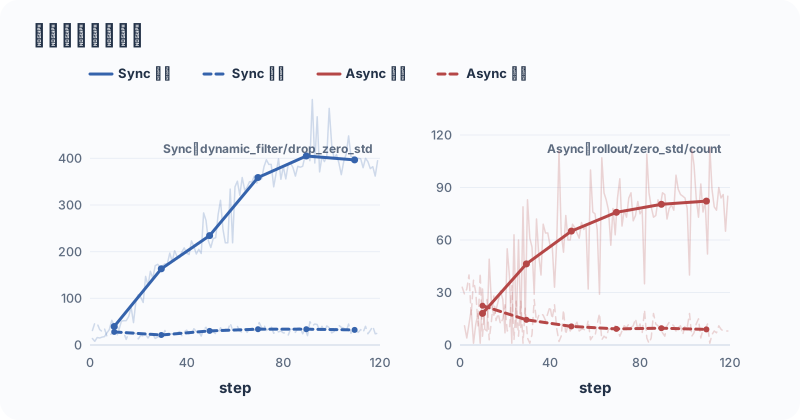
Besides reward, the all-correct/all-wrong group counts are worth watching. Reward only reflects how the model does across all problems, but note: in GRPO, a group that’s all-correct or all-wrong means $\sigma_R=0$ within the group — the whole group produces no gradient signal (recall the DAPO dynamic sampling section). In the left plot, Sync’s counterpart is dynamic_filter/drop_zero_std_1 (the number of groups dropped per step for being all-correct — Sync has dynamic-sampling filtering enabled), rising from 14 to 400: late in training, to assemble a batch of valid groups, the inference side throws away hundreds of all-correct groups per step — exactly the situation where dynamic sampling needs to roll out significantly more samples once hard-enough problems run short. When this curve keeps climbing, it’s time to consider switching to a harder problem bank or adjusting the sampling distribution.

Also worth a glance is the old familiar grad_norm — though in both of my runs it was flat, with no spikes and no NaNs.

Staleness and TIS

The async logs contain a set of metrics the sync run lacks, matching the staleness and TIS theory from earlier:

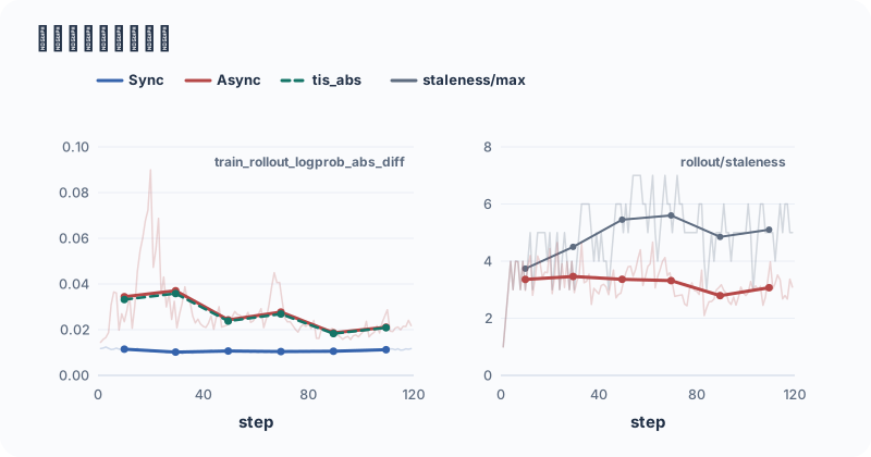
• rollout/staleness/mean ≈ 3–3.5: by the time each data point is consumed by training, the training side has on average advanced 3 more versions since sampling; the single-step maximum is 4.7, and staleness/max has peaked at 7. This is the version lag that fully async buys with throughput.
• train/tis / train/tis_abs / train/tis_clipfrac: the mean of the TIS weight $w=\pi_{\mathrm{train}}/\pi_b$ is almost exactly 1.0000. But a mean of 1 absolutely does not mean no drift — 0.9 and 1.1 also average to 1. The real drift magnitude shows up in tis_abs (i.e., $\operatorname{mean}(|w-1|)$, around 2%–3.6% throughout); tis_clipfrac peaks at only 0.5%, meaning extreme outlier weights are rare.
• The left plot shows Async’s logprob_abs_diff running higher than Sync’s. Under async, this value is the superposition of numerical mismatch and policy staleness.

Efficiency: Where Async Actually Wins

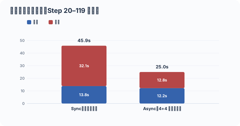
Per-step time dropped by $45.9/25.0\approx 1.84\times$, while training itself barely got faster (13.8s → 12.2s) — nearly all the savings are waiting: while the training side digests the previous batch, the inference side keeps producing the next one. Note that async’s generation length is even longer than sync’s, yet the overall step is still faster — clear evidence of substantial gains.

Closing Thoughts

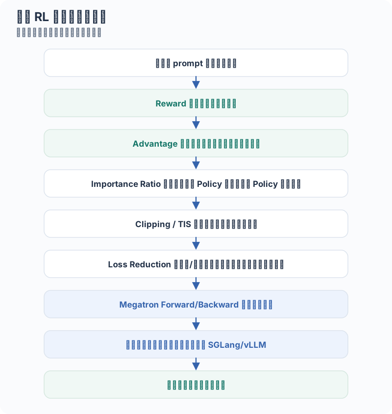
Reduce the whole RL workflow back to the real system loop, and this is the clear pipeline you get: